Introduction
In the first part of this series, we walked through an example of using PyTorch to do linear function fitting. In this part, we will see how to use a "neural network" model. The example will only require a few modifications to the examples from the previous post.
As I mentioned in the first post, machine learning if fundamentally function optimization. Recently, neural networks have become popular, and are almost synonymous with machine learning, but they are not really the same thing. Neural networks are a type of function that can be used to approximate the function we are looking for.
Simple Linear Neural Network
Creating the Model
To start, let's use the same training data that we used last time. We had four x-y pairs taken from the line $y = 2x + 1$.
data = [ [0,1], [1,3], [2,5], [3,7] ]
print(data)
# outputs:
# [[0, 1], [1, 3], [2, 5], [3, 7]]
Again, we need to import the torch module, and then we can define our model.
import torch

class NNet(torch.nn.Module):
  def __init__(self):
    super().__init__()
    self.l1 = torch.nn.Linear(in_features=1,out_features=10)
    self.l2 = torch.nn.Linear(in_features=10,out_features=1)

  def forward(self,x):
    x = self.l1(x)
    return self.l2(x)
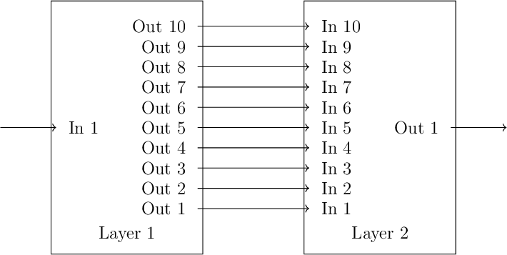
Here again, our model takes one input and computes one output, but this time we are using two linear models, or layers. Layer 1 (l1) takes one input and computes 10 outputs. Layer 2 (l2) takes
10 inputs and computes 1 output. We "connect" these layers together by feeding the outputs of layer 1 into the inputs of layer 2. That is our neural network (note: this won't be a very good
network, because it is still linear, but we'll talk about that later). Here is a very bad illustration
Everything else is the same as before. We create an instance of the model and print the initial parameter values.
fit = NNet()

print("initial parameters")
for p in fit.parameters():
  print(p)
# outputs:
# initial parameters
# Parameter containing:
# tensor([[-0.7987],
#         [ 0.0862],
#         [ 0.6410],
#         [ 0.7640],
#         [-0.8097],
#         [ 0.3653],
#         [ 0.8412],
#         [-0.6387],
#         [ 0.6078],
#         [-0.3472]], requires_grad=True)
# Parameter containing:
# tensor([-0.0951,  0.2870,  0.4422,  0.7289,  0.4854, -0.1306, -0.3795,  0.6540,
#         -0.2433, -0.3002], requires_grad=True)
# Parameter containing:
# tensor([[-0.1362, -0.1951, -0.1765, -0.2165,  0.1072,  0.3011, -0.2424,  0.0349,
#           0.2938, -0.2380]], requires_grad=True)
# Parameter containing:
# tensor([-0.2853], requires_grad=True)
This is a little different than before. There are four model parameters this time, and they aren't all the same shape. To make sense of this, we need to consider what the linear model is actually doing with its inputs. Let's look at the last two parameters first. These are the parameters in layer 2. Recall in the previous post, we used a linear model to do quadratic regression by treating $x$ and $x^2$ as separate inputs. If we define $x_1 = x^2$ and $x_2 = x$, then the model parameters consist of the coefficients for each input, call these $p_1$ and $p_2$, plus the y-intercept, call this $b$. The model output calculation can then be written in matrix form. $$ y = \left( \begin{matrix} p_1 & p_2 \end{matrix} \right) \left( \begin{matrix} x_1 \ x_2 \end{matrix} \right) + b $$ If you go back and look at the model parameters for the quadratic fit, there were two listed. One was a two element "row" tensor (this would be the $(p_1 \; p_2)$ matrix), and the other was a single element tensor (this would be $b$). For a linear model taking 10 inputs, this becomes $$ y = \left( \begin{matrix} p_1 & p_2 & p_3 & p_4 & p_5 & p_6 & p_7 & p_8 & p_9 & p_{10} \end{matrix} \right) \left( \begin{matrix} x_1 \ x_2 \ x_3 \ x_4 \ x_5 \ x_6 \ x_7 \ x_8 \ x_9 \ x_{10} \end{matrix} \right) + b $$ So, the last parameters shown (with value -0.2853) is the y-intercept. The second-to-last parameter shown is the 10 element coefficient matrix. What about a model that takes one input and produced two outputs? In matrix form, this would be written $$ \left( \begin{matrix} y_1 \ y_2 \end{matrix} \right) = \left( \begin{matrix} p_1 \ p_2 \end{matrix} \right) x + \left( \begin{matrix} b_1 \ b_2 \end{matrix} \right) $$ Now we have two coefficients, and two y-intercepts (or "bias" terms). For a model that produces 10 outputs, we would have 10-element matrices instead. This is what the first two model parameter are. In general, a linear model can take $n$ inputs and produce $m$ outputs. In this case, we would have and $n\times m$ tensor parameter for the coefficients, and an $1\times m$ tensor for the y-intercepts.
Now we understand the model parameters. Let's use the model to compute an output.
x = torch.FloatTensor([1])
y = fit(x)
print("initial prediction",x,y)
# outputs:
# initial prediction tensor([1.]) tensor([-0.5649], grad_fn=<AddBackward0>)
It's not as easy to check in this case, but the model output is just multiplying the input (1) by each of the coefficients, adding them together, and then adding the y-intercept.
Training the Model
We are now ready to train out model. The training looks exactly as it did in the linear regression case.
x = []
y = []
for i in range(len(data)):
  x.append([data[i][0]])
  y.append([data[i][1]])
x = torch.FloatTensor(x)
y = torch.FloatTensor(y)

for i in range(100000):
  pred = fit(x)
  loss = calc_loss(pred,y)
  loss.backward()
  optimizer.step()
  optimizer.zero_grad()

print("final parameters")
for p in fit.parameters():
  print(p)
# outputs:
# final parameters
# Parameter containing:
# tensor([[-1.5818],
#         [-0.0890],
#         [ 0.9125],
#         [ 1.1311],
#         [-1.0611],
#         [ 1.0562],
#         [ 0.9274],
#         [-0.8444],
#         [ 1.4221],
#         [-1.0394]], requires_grad=True)
# Parameter containing:
# tensor([ 0.1331,  0.2398,  0.2289,  0.4636,  0.6944, -0.2168, -0.6082,  0.8025,
#         -0.3929, -0.1937], requires_grad=True)
# Parameter containing:
# tensor([[-1.5220, -0.1104,  0.8442,  1.0497, -0.9803,  1.0463,  0.8340, -0.7835,
#           1.3899, -1.0276]], requires_grad=True)
# Parameter containing:
# tensor([-0.0602], requires_grad=True)
Here we can see that the model parameters have been updated, but are they correct?
With a neural network, we can't tell by just looking at the model parameters. The point of the network is not to predict coefficients that have some meaning, the point is to predict the correct output for a given input. So all we can do is "validate" that our model produces the expected outputs for some set of inputs. Let's feed the model the training data.
y = fit(x)
print("final prediction",x,y)
# outputs:
# final prediction tensor([[0.],
#         [1.],
#         [2.],
#         [3.]]) tensor([[1.0000],
#         [3.0000],
#         [5.0000],
#         [7.0000]], grad_fn=<AddmmBackward>)
So the model exactly replicates the training data. Let's try a few other points. Recall that the data is sampled from the line $y = 2x + 1$. So the model should also produce $(2.5,6)$ and $(10,21)$. Add the following lines to the end of the file.
x = tensor.FloatTensor([ [2.5], [10] ])
y = fit(x)
print("new prediction",x,y)
# outputs:
# new prediction tensor([[ 2.5000],
#         [10.0000]]) tensor([[ 6.0000],
#         [21.0000]], grad_fn=<AddmmBackward>)
The model correctly predicts these outputs too, so all looks good. However...
The model we have build is still linear. We are feeding the outputs of a linear function into the inputs of another linear function. Here we are passing 10 values between layer 1 and 2, but let's consider a simpler case first. If we passed just two parameters between the layers, then in matrix form, our model would look like this $$ y = \left( \begin{matrix} p_{2,1} & p_{2,2} \end{matrix} \right) \left[ \left( \begin{matrix} p_{1,1} \ p_{1,2} \end{matrix} \right) x + \left( \begin{matrix} b_{1,1} \ b_{1,2} \end{matrix} \right) \right] + b_{2,1} $$ The term in square brackets [] is layer 1 applied to the input $x$. This is fed into layer 2 as a column vector, which computes a single value $y$. This is just a matrix equation, which means it is linear. $y$ will be a linear function of $x$, which means we cannot represent non-linear functions. This is certainly not what we want, we could just use a linear model for that.
Let's use the quadratic training data from the last post with points sampled from $y = 3x^2 + 2x^2 + 1$.
#data = [ [0,1], [1,3], [2,5], [3,7] ]
data = [ [0,1], [1,6], [2,17], [3,34] ]
Rerunning the model will print something similar to
final prediction tensor([[0.],
        [1.],
        [2.],
        [3.]]) tensor([[-2.0000],
        [ 9.0000],
        [20.0000],
        [31.0000]], grad_fn=<AddmmBackward>)
new prediction tensor([[ 2.5000],
        [10.0000]]) tensor([[ 25.5000],
        [108.0000]], grad_fn=<AddmmBackward>)
So here the model is not even able to correctly predict the training data. That's because it is trying to find a straight line that passes through a curve. Evidently, the line it has "learned" is $y = 11x - 2$.
Non-Linear Neural Network
In order for our neural network to learn a non-linear function, we have to add some non-linearity. This is done by passing the outputs of layer 1 through a non-linear function before passing them to layer 2. This function is called the "activation function". The specific non-linear function we use could be any non-polynomial, but there are a few common choices.
- tanh - the hyperbolic tangent function.
- sigmoid - any function that has a characteristic "S" shape. tanh is one example of such a function.
- relu - "rectified linear unit", a simple non-linear function that is easy to compute and seems to work.
So, with our activation functions in place, we will have something like this.

The red dots represent our activation function, which can be any non-linear function. There is no clear choice in what we should use for our activation function. It depends on the problem, and is something that we generally have to try and see how it works. For now, let's use tanh. We update our model to apply the activation function to layer 1's outputs before feeding them into layer 2's inputs.
class NNet(torch.nn.Module):
  def __init__(self):
    super().__init__()
    self.l1 = torch.nn.Linear(in_features=1,out_features=10)
    self.l2 = torch.nn.Linear(in_features=10,out_features=1)

  def forward(self,x):
    x = self.l1(x)
    x = torch.tanh(x)
    return self.l2(x)
Now if we rerun the example, we get something similar to this.
final prediction tensor([[0.],
        [1.],
        [2.],
        [3.]]) tensor([[ 1.0000],
        [ 6.0000],
        [17.0000],
        [34.0000]], grad_fn=<AddmmBackward>)
new prediction tensor([[ 2.5000],
        [10.0000]]) tensor([[27.2216],
        [38.5437]], grad_fn=<AddmmBackward>)
Our model has exactly predicted our training data. However, it does not give the correct output for different inputs. For $x = 2.5$, $y = 24.75$, but our model predicts 27.2216. Similarly, for $y(10) = 321$, but our model predicts 38.5437. This highlights two points. First, if we know that our data should fit a quadratic function, then we should just use a quadratic model. Our neural network is trying to learn that our data is quadratic, but it does not have enough training data to do so. Second, we can't be certain that our trained model will extrapolate to values outside the training data. We would like for this to be the case, but we will have to validate that this is the case.
Closing
That's basically all there is to neural networks. We take the output of a linear model, apply a non-linear function, and feed them into another linear model. Of course, we can construct more complicated networks. If we use more than two layers,
class NNet(torch.nn.Module):
  def __init__(self):
    super().__init__()
    self.l1 = torch.nn.Linear(in_features=1,out_features=10)
    self.l2 = torch.nn.Linear(in_features=10,out_features=1)
    self.l3 = torch.nn.Linear(in_features=10,out_features=1)

  def forward(self,x):
    x = self.l1(x)
    x = torch.tanh(x)
    x = self.l2(x)
    x = torch.tanh(x)
    return self.l3(x)
then we have a "deep" neural network. The example given here is not well suited for a neural network. Our function was pretty simple, and we didn't have very much training data. Neural networks are useful for approximating very complex functions with many inputs. They are popular for classifying images, for example. We can think of them as providing us with lots of knobs to adjust so that we can approximate lots of different functions. However, with more knobs to adjust, we need more training data to correctly adjust the knobs. They have become popular in recent years now that we have the data sets, and computational power to train them.